Adaptive Trees on a GPU: Efficient GPU-aware Adaptive Tree Construction for the Fast Multipole Method

Nils Rottstegge^1,2
1Department of Computer Science, ETH Zürich · ²Jülich Supercomputing Centre (JSC), Forschungszentrum Jülich, Guest Student Programme 2026 (August – October 2026)

Abstract. The Fast Multipole Method (FMM) reduces the cost of long-range particle interactions from $\mathcal{O}(N^2)$ to $\mathcal{O}(N)$, but its performance depends strongly on the spatial hierarchy it operates on. Dense trees are regular but waste work on empty space, while pointer-based sparse trees follow the particles but are irregular and hard to update on a GPU. This report presents a GPU implementation of adaptive trees for the FMM based on the Cornerstone representation, in which a tree is a sorted array of space-filling-curve boundaries and every update is a sequence of bulk-parallel array primitives. It introduces NFCount, a refinement criterion that adapts the tree to the expected near-field work instead of the particle density, and a traversal-free reconstruction of the explicit FMM hierarchy from the boundary array. A series of GPU optimisations, including cooperative stencil evaluation, cached recomputation, allocation-free buffer management and CUDA Graph replay with device-owned state, makes repeated updates cheap. The final implementation updates the tree and builds the FMM view up to 2.4× faster than Cornerstone while producing considerably more output, and accelerates the complete FMM pipeline by up to 4.8× compared with a dense tree. Finally, the approach is generalised to a binary adaptive tree with longest-side splits.

Keywords: fast multipole method, adaptive octree, space-filling curves, GPU, CUDA Graphs, k-d tree

Interactive figures

Most figures are interactive. Use ◀ ▶ to step through algorithms, drag the sliders, hover arrays and click plots to enlarge them. The algorithm figures run small JavaScript models of the kernels, so numbers shown in them belong to toy examples. All measurements come from the benchmark suite described in Section 7.

1. Introduction

Particle simulations in molecular dynamics, plasma physics and astrophysics are dominated by long-range interactions between all pairs of particles. Evaluating these pairs directly costs $\mathcal{O}(N^2)$ operations per time step, which is infeasible for millions of particles and thousands of steps. The Fast Multipole Method (FMM) [1] reduces this cost to $\mathcal{O}(N)$ by grouping particles in a spatial hierarchy and letting well-separated groups interact through series expansions.

The structure of this hierarchy determines the balance between near-field and far-field work. Large leaves cause many expensive direct interactions, while small leaves cause many boxes and expansion translations. For non-uniform distributions, such as an expanding Coulomb explosion or a thin disk in an otherwise empty domain, a uniform tree is either too coarse where the particles are or wastes most of its boxes on empty space. An adaptive tree refines only where it is needed.

On a GPU, adaptivity comes at a price. Pointer-based trees are irregular, require dynamic allocation and are difficult to build in parallel. In a time-stepping simulation the tree additionally has to follow the particles every step, so construction is a recurring cost. If updating the tree takes as long as the FMM saves, nothing is gained.

This project builds on the Cornerstone library [2], which represents an adaptive octree as a sorted array of space-filling-curve keys and updates it with bulk-parallel primitives. The FMM code used at JSC, FMSolvr [3], however needs an explicit hierarchy with a specific node layout, per-node particle ranges and a particle-to-leaf mapping, and ideally a tree that is refined according to the work the FMM will actually perform. This report makes the following contributions:

1. NFCount, a refinement criterion based on the estimated near-field work of a leaf and its 27-cell neighbourhood (Section 3.3).
2. A direct TreeView construction that derives all internal nodes and their final positions in FMSolvr's layout from the boundary array, without tree traversal (Section 4).
3. A series of GPU optimisations that make repeated updates cheap, culminating in a CUDA-Graph-compatible update (Section 5).
4. A binary adaptive tree that reuses the same representation and view construction (Section 6).

Section 2 introduces the FMM, adaptive trees and the Cornerstone representation. Sections 3 to 6 present the methods, Section 7 the experimental setup and Section 8 the results. Section 9 outlines future work and Section 10 concludes.

2. Background

2.1 The Fast Multipole Method

The FMM [1] [4] organises the particles in a hierarchy of nested boxes. The interaction between two groups of particles that are well separated, i.e. far apart compared to their size, is approximated by truncated multipole and local expansions. Figure 1 shows the resulting operators.

P2M · M2M	upward: particles → multipoles → parents
M2L	far field between well-separated nodes
L2L · L2P	downward: parents → children → particles
P2P	direct near field between neighbouring leaves

The FMM operators on a small tree. Upward pass: particles to multipoles (P2M) and children to parents (M2M). Far field between well-separated boxes (M2L). Downward pass: parents to children (L2L) and to particles (L2P). Near field: direct interactions between neighbouring leaves (P2P).

The cost splits into two parts with opposite dependence on the tree. The far field scales with the number of boxes and the expansion order. The near field scales with the number of particle pairs in neighbouring leaves and grows quadratically with the leaf occupancy. Refining a leaf therefore trades near-field work for far-field work, and a good tree balances the two locally. Since multipoles are passed up and local expansions down through all internal nodes, the FMM also needs the full hierarchy, not only the leaves.

2.2 Dense, Sparse and Adaptive Trees

Figure 2 compares three ways to build the resulting tree. A dense tree subdivides the whole volume to the same depth. Its layout is perfectly regular and GPU-friendly, but empty boxes are stored and processed and the depth cannot follow the local density. A sparse tree stores only occupied boxes, typically linked by pointers. It is memory-efficient, but pointer chasing, scattered accesses and dynamic allocation map poorly to GPUs. An adaptive tree refines dense regions and keeps coarse cells elsewhere. As the following sections show, it can be stored in contiguous arrays and updated with regular parallel primitives.

Dense

341 nodes256 leaves220 emptydepth 4

Sparse

59 nodes36 leaves0 emptydepth 4

Adaptive

113 nodes85 leaves17 emptydepth 6

Toy 2D examples on the same particles. Left: dense tree (grey = empty cells). Middle: sparse tree storing only occupied cells. Right: adaptive tree (shade = depth).

2.3 Space-Filling Curves and the Cornerstone Representation

A pointer-free tree requires an address for every cell. Each particle position is quantised onto an integer grid and the coordinate bits are interleaved into a Morton key. In the 3D octree, every three bits select one of eight children on the next level, so a cell at level $\ell$ owns exactly the contiguous interval of keys that share its first $\ell$ three-bit digits. Figure 3 illustrates the same principle in 2D using a quadtree, where each level contributes two bits instead. Sorting particles by key therefore groups them by cell on every level at once. With 64-bit keys, the octree supports 21 levels, and a level-$\ell$ cell spans an interval of width $r_{\ell }=2^{63-3\ell }$.

show Z-curve (key order)

x = 5101

y = 2010

interleave ↓ (x bit, y bit) per level

key100110= 38

digitsL1: 2L2: 1L3: 2

Each 2-bit digit selects a quadrant one level deeper (dashed squares). A cell at level ℓ therefore owns the contiguous key interval that shares its first ℓ digits. This is what makes a tree representable by sorted keys alone.

Morton keys in 2D. Hover a cell to see its x and y bits interleave into the key. Each 2-bit digit selects one quadrant (dashed boxes). The line shows the Z-shaped key order.

After key generation, the particles are radix-sorted as key/permutation pairs. P holds the sorted keys and Perm[p] the original slot of the particle at sorted position p. Note that numerical proximity of keys does not imply geometric proximity, since neighbouring cells across a high-level boundary can have very different keys. Neighbour queries therefore have to be formulated geometrically (Section 3.3).

Cornerstone [2] stores an adaptive tree only by the boundaries of its leaves, which partition the key space into consecutive intervals:

$$K=[k_0,k_1,\dots ,k_L],\text{leaf }i=[K_i,K_{i+1}).$$

A short interval corresponds to a deep, small leaf and a long interval to a coarse leaf. The array contains neither internal nodes nor pointers. Together with the particle counts $N_i$, obtained by two binary searches of $K_i$ and $K_{i+1}$ in P, it forms the complete state that is kept between time steps. Every split replaces a leaf by all eight children, including empty ones, so the represented tree is a full octree. This property is essential for the node-count formulas in Section 4. Figure 4 shows how $K$ evolves as a toy tree is refined.

1/4 · root: K = [0, 64]

K =064

root · 1 leaves → K has 2 entries · hover a leaf

The Cornerstone array K for a toy 2D quadtree with keys at coarse resolution (0 … 64). Each split replaces one interval by four (in 3D: eight) equal sub-intervals. Hover a leaf to see its interval, level and particles.

3. Adaptive Tree Update

3.1 Parallel Rebalancing

An update decides for every leaf independently whether it should split, stay or merge with its seven siblings. Each decision is encoded as the number of output leaves (8, 1 or 0). An exclusive prefix sum over these numbers yields the output position of every leaf, after which all threads write their new boundaries independently. A rebalance pass thus consists of three bulk-parallel steps: decide, scan and scatter. Figure 5 illustrates one pass on a toy octree with 22 leaves that is reused throughout this report.

1/5 · K and counts N

LeafCount threshold 8· 22 leaves, 29 particles · key space [0, 512)

Leaf i owns the key interval [K[i], K[i+1]). Shade = depth. Red counts exceed the threshold. Hover a leaf to highlight its particles.

One rebalance pass on a toy octree with 22 leaves, 29 particles and key space [0, 512), i.e. three octree levels. With a threshold of 8, two leaves split and eight siblings merge, resulting in 29 leaves. Move the threshold to change the decisions.

A merge is encoded implicitly. The first sibling contributes one boundary and the other seven contribute none, so the remaining boundary extends over the whole parent. An operation of 1 therefore either keeps a leaf or marks the leader of a merge, a distinction that becomes important for caching in Section 5.2. Heavily overfull leaves are split by several levels at once (64, 512 or 4096 children), which saves complete decide, scan and scatter rounds:

...
    if (count > bucketSize * 512 && level + 3 < maxTreeLevel<KeyType>{})
        return 4096;
    if (count > bucketSize * 64 && level + 2 < maxTreeLevel<KeyType>{})
        return 512;
    if (count > bucketSize * 8 && level + 1 < maxTreeLevel<KeyType>{})
        return 64;
    if (count > bucketSize && level < maxTreeLevel<KeyType>{})
        return 8;
...

Source: src/octree/octree_rebalance.cuh, commit d830fc3, lines 215–225.

For NFCount the jump thresholds grow by a factor of 64 instead of 8 per level, since the occupancy drops by about 8 per level and the quadratic interaction work by about 64.

3.2 Incremental Updates

Because $K$ retains the previous topology, an update starts from the tree of the previous time step instead of from the root. Particles are re-keyed and re-sorted, the counts are refreshed, and rebalance passes are applied until the tree no longer changes (Figure 6). Since particles move only slightly between steps, one or two passes are usually sufficient.

One time step. Key generation and sorting, the rebalance cycle, TreeView construction and the FMM. Blue marks the tree-update phase and orange the view construction.

3.3 FMM-aware Refinement: NFCount

Cornerstone’s criterion, LeafCount, splits a leaf when it contains more than a fixed number of particles. For the FMM, this criterion is extended to account for the surrounding particle distribution. The cost caused by a leaf is dominated by its near field, i.e. the direct interactions of its particles with all particles in neighbouring boxes. A leaf with few particles next to a dense cluster can therefore be far more expensive than its own particle count suggests. NFCount estimates this work as

$$W_i=n_i,S_i,S_i=\sum _{\delta \in {-1,0,1}^3}n(C_i+\delta ),$$

where $n_i$ is the number of particles in leaf $i$, $C_i$ denotes its cell at the same refinement level, and $n(C)$ is the number of particles contained in cell $C$. The offset $\delta =({\delta }_x,{\delta }_y,{\delta }_z)$ enumerates the $3\times 3\times 3$ stencil around $C_i$, so $S_i$ is the total number of particles in the 27 same-level cells surrounding and including the leaf. Thus, $W_i$ estimates the number of direct particle interactions associated with leaf $i$.

For a uniformly populated neighbourhood, where each stencil cell contains approximately $n_i$ particles, $S_i\approx 27n_i$ and hence $W_i\approx 27n_i^2$. This motivates the default threshold

$$W_{\max }=27\cdot {64}^2=110,592,$$

which corresponds to the near-field work of a uniformly populated neighbourhood with the LeafCount default of 64 particles per cell. Figure 7 compares both criteria on the same leaf.

3D: leaf + 26 same-level neighbours

LeafCount · particles in the leaf

N_i = 7

NFCount · leaf + 3×3 same-level stencil

NF_i = 7 · (7 + 268) = 1925

same leaf in both panels · hover another leaf · 2D toy: 3×3 stencil (3D: 3×3×3)

LeafCount only considers the particles inside the leaf, NFCount its 3×3 (in 3D: 3×3×3) same-level neighbourhood. Hover other leaves: sparse leaves next to clusters become expensive under NFCount.

Counting geometry instead of leaves. The first implementation 1755802 searched neighbours in the leaf array and only accepted a leaf of exactly the same level. Wherever the neighbourhood was represented by coarser or finer leaves, its particles were missed, and only a directional subset of the stencil was evaluated. The final version e7bd16a instead queries the particles. Each stencil cell is a key interval $[k_c,k_c+r_{\ell })$, and its population follows from two binary searches,

$$n_c=\mathrm{lowerBound}(P,k_c+r_{\ell })-\mathrm{lowerBound}(P,k_c),$$

which is correct regardless of how the tree is refined around the leaf.

Merging. Eight siblings may only merge if their hypothetical parent stays below the threshold. Since the parent has a larger stencil, its work cannot be derived from the children's values and is evaluated explicitly, once per sibling group 6f11cac.

A naive evaluation of NFCount requires 54 binary searches per leaf, with two searches for each of the 27 stencil cells. In comparison, LeafCount requires only two binary searches per leaf. Reducing this overhead is the subject of Section 5.

4. TreeView Construction

$K$ is well suited for adaptation, but the FMM cannot operate on it directly. The upward and downward passes require internal nodes, parent and child links, level offsets, per-node particle ranges and a mapping from particles to leaves (Figure 8). We refer to these arrays as the TreeView. Compared with Cornerstone, the view additionally contains NF values, per-node particle counts and offsets, and the particle-to-leaf map, all in the layout expected by FMSolvr [3] (Figure 9).

The FMM needs the full hierarchy. Leaves correspond to intervals of K, whereas internal nodes (dashed) are not stored and must be reconstructed.

computeSfcKeys · sort · updateOctreeGpu · buildOctreeGpu

adaptive update · TreeView

inner ring: tree-update phaseview phasenot computed

Outputs of Cornerstone and of this work, grouped by kind. The inner ring shows whether an array is produced in the tree-update phase (blue) or the view phase (orange). Hatched arrays are not computed by Cornerstone.

4.1 Child-Centric Layout

FMSolvr stores the nodes level by level and expects the children of a level in child-centric order: first child 0 of every parent, then child 1 of every parent, and so on 3c99271. With $M$ internal parents on a level, the children of parent $p$ are located at

$$\mathrm{child}(p,c)=\mathtt{\text{childIndex}}[p]+c\cdot M,$$

where $p$ identifies the parent, $c\in 0,\dots ,7$ is the child slot, and $M$ is the number of internal parents on that level. Thus, childIndex[p] points to child 0 rather than to a block of eight contiguous children (Figure 10).

parents M 3

A = node 6B = node 7C = node 8

A09

B010

C011

A112

B113

C114

A215

B216

C217

A318

B319

C320

A421

B422

C423

A524

B525

C526

A627

B628

C629

A730

B731

C732

hover a child slot

childIndex[p] always points to child 0. With level offsets known, M = (levelOffset[ℓ+2] − levelOffset[ℓ+1]) / 8, so no per-node child list is needed.

Parent-major versus child-centric layout. Hover a child to see how its index is computed.

4.2 From Breadth-First Search to Direct Reconstruction

The child-centric layout introduces a dependency between consecutive levels. To place the children of a level, the number of internal parents $M$ on the preceding level must be known. A straightforward construction therefore uses a breadth-first traversal. It processes one level, determines how many internal nodes it contains, and then uses this count to place the children on the next level. On the GPU, this requires synchronization between levels and prevents the hierarchy from being constructed in a single parallel step.

The view construction went through four versions. The first c4719cd copied $K$ to the host, built the tree recursively and uploaded the result. The second used a breadth-first traversal on the CPU, which naturally provides the per-level node counts required by the child-centric layout 3c99271. The third moved this traversal to the GPU c7774e2. It avoided host round trips, but retained the level-by-level dependency. Every level required synchronization and repeated clears, scans and launches sized for the whole tree, while most threads had no work on a given level.

The fourth version 8041613 eliminates the traversal altogether. Instead of discovering the hierarchy and its per-level sizes level by level, it derives them directly from the leaf boundaries in $K$. This is possible because the required sizes and the internal nodes can both be determined analytically, based on two observations.

All sizes are known in advance. Every internal node has eight children and every node except the root has exactly one parent. Counting edges gives for $L$ leaves

$$8I=(L+I)-1⟹I=\frac{L-1}{7},$$

and in general $I=(L-1)/(2^b-1)$ for $b$ bits per level. Working upwards from the deepest level, the per-level counts follow from $I_{\ell }=T_{\ell +1}/8$ and $T_{\ell }=L_{\ell }+I_{\ell }$, where $L_{\ell }$ and $T_{\ell }$ denote the leaves and all nodes on level $\ell$.

Every internal node corresponds to exactly one boundary in $K$. Between the subtrees of its child 0 and child 1 lies exactly one leaf boundary. For each boundary, the lowest common ancestor of the two adjacent leaves is computed. If the right leaf lies in child slot 1 of that ancestor, the boundary identifies one internal node:

const KeyType leftStart = K[i];
const KeyType rightStart = K[i + 1];
const unsigned level = lcaLevel<LevelBits>(leftStart, rightStart);
const KeyType parentStart =
    nodeStartAtLevel<LevelBits>(rightStart, level);
const unsigned rightChild =
    childSlotAtLevel<LevelBits>(rightStart, parentStart, level + 1);
// For either full tree, rightChild == 1 means this
// boundary is exactly:
//
//     child0 subtree | child1 subtree
const bool canonical = (rightChild == 1);

Source: src/common/tree_view.cu, commit d830fc3, lines 185–199 (abridged).

In the toy octree of Figure 5, boundary 64 identifies the root and boundaries 8 and 136 identify root children 0 and 2. The leaf histogram per level $[0,6,16]$ yields $[1,2,0]$ internal nodes and $22+3=25$ nodes in total, in agreement with $I=(22-1)/7$.

The remaining stages compact the flagged candidates, sort them, and write every node directly to its final position

$$\text{idx}=\mathtt{\text{levelOffset}}[\ell ]+\text{childSlot}\cdot M_{\ell -1}+m_{\text{parent}},$$

where $m_{\text{parent}}$ is the rank of the parent within its level. Internal nodes and leaves are written by independent kernels. Figure 11 walks through all stages on a small example.

1/5 · input K, sizes known analytically

Input: Cornerstone K

0481216323640444864

L = 10 leaves. Every internal node has 2^b = 4 children ⇒

#internal = (L − 1) / (2^b − 1) = 3

sizes are known analytically, before building anything.

Direct construction on a toy K with four children per node (the implementation uses eight for the octree and two for the binary tree). The final step shows the flat node array in child-centric order.

4.3 One Sort Instead of Two

The child-centric order requires internal nodes sorted by level and, within a level, by their child path read backwards. The first direct implementation used two radix sorts. Commit 8e958d5 combines both criteria into a single key,

$$q=(1\ll 3\ell )|\text{reversedPath}.$$

Since the reversed path of a level-$\ell$ node is smaller than $2^{3\ell }$, the marker bit assigns every level a separate numeric range, and a single sort yields the same order (Figure 12). The same commit also folds the parent-pointer writes into the internal-node kernel and removes a separate kernel.

1/4 · SFC order (input)

#	node path	level	reversed path
0	root	0	— (0)
1	0	1	0 (0)
2	0·3	2	3·0 (24)
3	0·7	2	7·0 (56)
4	2	1	2 (2)
5	2·1	2	1·2 (10)
6	2·6	2	6·2 (50)

Internal nodes in level-grouped SFC order (what the classify/compact stages produce). Paths are octal child digits from the root.

Internal nodes of a small octree. Steps 1 and 2 show the original two-sort approach, step 3 the single sort on the combined key.

Particle ranges. The particle range of a leaf requires no search, since the leaf counts are already known. An exclusive scan over $N$ yields the begin offsets c2f2cbf, and leaf $i$ owns $P[B_i:B_i+N_i]$ with $B_i=\sum _{j<i}{N}_j$.

5. GPU Optimisations

The previous sections define what is computed. Most of the project time went into how it is computed on the GPU. Figure 13 shows the 34 commits of the repository. They fall into four phases: making the tree usable for the FMM (late August), making NFCount correct and parallel (early September), avoiding repeated work (mid September) and removing the CPU from the update path (second half of September), followed by the binary tree.

Hover or click a commit. ★ = milestones that changed the performance picture.

Commit timeline of the repository. Hover or click a commit for details, or filter by theme. ★ marks milestones that changed the performance picture.

5.1 Cooperative Stencil Evaluation

Instead of one thread evaluating all 27 cells, a cooperative group of eight threads shares one leaf e7bd16a. Lane $t$ processes cells $t$, $t+8$, $t+16$ and $t+24$, and the partial sums are combined with warp shuffles (Figure 14). The centre cell's count equals the leaf's own particle count, so the kernel also produces $N$ without a separate counting pass c2f2cbf.

1/9 · assign cells to lanes

numbers = particles in each same-level geometric cell · #13 = the leaf itself

lane	cells	partial sum
0	0, 8, 16, 24	0
1	1, 9, 17, 25	0
2	2, 10, 18, 26	0
3	3, 11, 19	0
4	4, 12, 20	0
5	5, 13, 21	0
6	6, 14, 22	0
7	7, 15, 23	0

8 threads cooperate on one leaf. Cell c goes to lane c mod 8.

One leaf evaluated by eight lanes: four loop rounds of two binary searches per cell, the shuffle reduction and the resulting NF value.

// 27 = 3x3x3 same-level neighborhood, including the node itself
for (int cell = tile.thread_rank(); cell < 27; cell += tile.size())
{
    int dx = cell % 3 - 1;
    int dy = (cell / 3) % 3 - 1;
    int dz = cell / 9 - 1;

    KeyType cellKey =
        (cell == 13) ? nodeStart
                     : sfcNeighbor<KeyType>(ibox, level, dx, dy, dz, isHilbert);

    std::size_t first = std::size_t(
        lowerBound(particleKeys, particleKeys + numParticles, cellKey) -
        particleKeys);
    std::size_t last = std::size_t(
        lowerBound(particleKeys, particleKeys + numParticles, cellKey + range) -
        particleKeys);

    unsigned long long population =
        static_cast<unsigned long long>(last - first);
    populationSum += population;
    if (cell == 13)
        centerCount = population;
}

populationSum += tile.shfl_down(populationSum, 4);
populationSum += tile.shfl_down(populationSum, 2);
populationSum += tile.shfl_down(populationSum, 1);

Source: src/octree/octree_rebalance.cuh, commit d830fc3, lines 579–634 (abridged).

This distributes the searches but does not reduce their number. The following optimisation does.

5.2 Caching and Compaction

Within one update pass over $K$ the particles do not move, only the topology changes. A leaf whose interval survives a rebalance pass therefore keeps its $N$ and $NF$, since a neighbour splitting next to it does not change the population of a geometric stencil cell 65b11a5. The scatter kernel copies the cached values along with the boundaries and marks only new cells as dirty, namely split children and merge leaders. CUB's DeviceSelect then compacts the dirty flags into a dense index list, so the cooperative kernels only process leaves that require work 6d19359. For $L$ leaves of which $D$ are dirty, the number of searches drops from $54L$ to $54D$. In the toy example of Figure 15, only 17 of 29 leaves have to be re-evaluated. In the later graph-compatible version, the compaction is replaced by a fixed-size launch in which clean leaves return early.

leaf0123456781624324048566472808896104112120128192256320384448

reuse N, NF········✓✓✓✓✓✓✓·········✓✓✓✓✓

nfDirty11111111000000011111111100000

selected01234567151617181920212223

NF queries without caching

54 × 29 = 1566

with dirty flags + compaction

54 × 17 = 918

saved binary searches

648

■ split children · ■ merge leader (new, larger cell that must be recomputed although its op is 1) · ■ identical interval → N and NF copied from the old arrays.

The rebalance pass of Figure 5. Only 17 of the 29 output leaves require a new NF evaluation. At the start of a new time step all counts are stale, so the first pass refreshes every leaf.

Launch configuration. Later commits adapted the launch configuration to each workload 8e958d5 1d220c6. LeafCount refreshes use one thread per leaf instead of an eight-thread group with a single busy lane, full refreshes skip the selection of the identity list, and the evaluation of the leaves and of the hypothetical parents runs on separate streams.

5.3 Memory Management

Every rebalance pass and time step changes the number of leaves and with it the size of many buffers, including $K$, $N$, $NF$, flags, scan outputs and all view arrays. A plain resize() causes two costs. If the capacity is exceeded, new memory is allocated and the data copied. If the vector grows within its capacity, every newly exposed element is value-initialised by a fill kernel, although the next kernel overwrites it anyway. The second cost does not disappear by reserving enough memory. Profiling a single snapshot showed 23 initialisation kernels while not a single allocation was required.

1/12

time step 1 · required size 1000

ordinary resize()alloc

exact capacity · value-initialises new elements

alloc 1init 1000host resize 1

resizeWithHeadroomalloc

+25 % capacity · resize(n, thrust::no_init)

alloc 1init 0host resize 1

prepared graph capacityalloc + capture

fixed storage · logical count lives on the device

alloc 1init 0host resize 1recapture 1

capacitylogical size (written by the kernel)newly exposed → value-initialised, then overwrittenallocation this step

The same sequence of required sizes under three policies. Orange elements are value-initialised and then overwritten, red frames mark allocations. Counters accumulate over the time steps.

Commit 65b11a5 therefore replaces all resizing in the tree, rebalance and view code by a helper that grows the capacity by 25% only when necessary, never shrinks it, and changes the logical size without initialisation:

template <class T>
void resizeWithHeadroom(thrust::device_vector<T> &buffer,
                        std::size_t required)
{
    if (required > buffer.capacity())
    {
        const auto extra = required / 4;
        const auto limit = buffer.max_size();

        // Add 25% without overflowing; reserve handles oversized requests.
        const auto capacity =
            required <= limit && extra <= limit - required
                ? required + extra
                : required;

        buffer.reserve(capacity);
    }

    buffer.resize(required, thrust::no_init);
}

Source: src/helpers.cuh, commit 65b11a5, lines 6–25.

Buffers whose initial contents matter, such as histograms and flags, are still cleared explicitly. Two smaller changes reduce memory traffic further. Key generation writes the identity permutation directly instead of launching a separate kernel, and the permutation uses 32-bit instead of 64-bit indices 1914b3d, which reduces the sort payload from 16 to 12 bytes per particle.

5.4 Overlapping Independent Work

Many stages depend on the same inputs but not on each other. In the view construction, for example, the scan over $N$ can run while the internal-node structure is derived, and the level metadata only depends on the classification. Persistent streams and events express these dependencies explicitly e7bd16a 8041613 (Figures 17 and 18).

Streams and events of the TreeView construction (logical order, not to scale).

particle-side work × 1makespan 13.5 vs serial 19.0 units

Hover a task to see the events it waits on. Durations are illustrative units, not measurements. Overlap creates an opportunity, it does not guarantee perfect concurrency on a busy GPU.

The same tasks scheduled on one stream and on four streams with event dependencies. Durations are illustrative. Increase the particle-side work to see the particle scan and mapping dominate.

5.5 CUDA Graphs

After these optimisations, a significant part of each update was no longer GPU work but coordination between CPU and GPU. After every pass the host read the new leaf count, decided whether the tree had changed, resized buffers, swapped pointers and launched the next kernels, leaving the GPU idle during each round trip. CUDA Graphs avoid this overhead by capturing a sequence of launches once and replaying it with a single call, provided that addresses and structure remain fixed. Commits f19e711 and 93b637d rebuild the update around this constraint. The leaf count, the convergence flag and the active input buffer are stored in a state struct on the device, and kernels select their input and output arrays themselves. A fixed number of passes is recorded, and kernels scheduled after convergence return immediately. All buffers are prepared for a fixed capacity, and a proposal that would exceed it is rejected before anything is written:

__global__ void graphCheckCapacityKernel(const std::int64_t *nodeOps,
                                         TreeNodeIndex leafCapacity,
                                         RebalanceState *state)
{
    if (state->converged)
        return;
    if (state->needsResize || !state->changed)
    {
        state->converged = 1;
        return;
    }
    const std::int64_t proposedLeaves = nodeOps[leafCapacity];
    if (proposedLeaves > leafCapacity)
    {
        // Reject the complete proposal: the old tree and its freshly
        // computed counts remain valid, with no partially applied splits.
        state->needsResize = 1;
        state->converged = 1;
        return;
    }
    state->newNumLeaves = TreeNodeIndex(proposedLeaves);
}

Source: src/octree/octree_rebalance.cuh, commit d830fc3, lines 1211–1232.

The old tree then remains valid, and growth and recapture happen outside the replay (Figure 19). Two costs remain: a status readback after each replay, and capacity-sized work such as the CUB scan that runs regardless of convergence. Moreover, the default of two passes per octree update does not always reach full convergence on rapidly changing data.

topology exceeds capacityfixed passes 3

One launch replays a fixed number of passes. RebalanceState on the device holds the leaf count, convergence flag and active A/B buffer. Kernels after convergence exit immediately (grey slivers), but the capacity-sized CUB scan still runs. An oversized proposal is rejected before anything is written; growth and recapture happen outside the replay.

Conceptual timeline of one update with illustrative durations. Host-driven: every pass waits for a device-to-host copy. Graph replay: one launch, passes run back to back. Enable the overflow to see the rejection, growth and recapture path.

Escaped particles. Particles that leave the domain would change the particle count and thus the buffer sizes inside the graph. Since 056d000 they keep their slot but receive the maximum key, so the sort moves them to the end of P and the device determines the active prefix (Figure 20).

input slot

key3756118449MAX271333

sorted P5913182733374461MAX

Perm1583790426

Click a slot to let that particle escape the domain. Active particles: 9 / 10 slots. The tree counts and views only see the active prefix, and escaped entries map to an invalid node index. Note that key generation and the sort still touch all slots.

Click a slot to let that particle escape. Its slot stays allocated, its key becomes MAX and moves to the end of the sorted array (red line = active count).

6. Binary Adaptive Trees

An octree split always halves all three axes. A region that only requires refinement in one direction, such as a thin sheet or a filament, still receives eight children. A binary tree splits one axis at a time. Three binary levels reproduce one octree level, but an adaptive binary tree can stop earlier or refine only selected branches (Figure 21).

Octree: one split creates eight cubes. Binary tree: on a cube, three levels of splits along the longest side create the same eight cubes, or stop earlier with slabs and columns.

The binary tree always splits the longest side at its midpoint [5]. Since all cells at a given depth then have the same shape, a single axis schedule describes the whole tree and also supports rectangular domains 806464e:

for (unsigned depth = 0; depth < maxBinaryDepth; ++depth)
{
    unsigned axis = 0;
    if (length[1] > length[axis]) axis = 1;
    if (length[2] > length[axis]) axis = 2;
    geometry.axis[depth] = std::uint8_t(axis);
    length[axis] *= 0.5L;
}

Source: src/kdtree3d/binary_node.cuh, commit d830fc3, lines 31–38.

The key encoding interleaves the coordinate bits in the same order, so every cell is again a contiguous key interval (Figure 22). The result is a linear kd-tree [6] on which the Cornerstone machinery carries over unchanged, including rebalancing, device state and capacity handling. The direct view construction only relies on every internal node having a unique boundary between its first two subtrees, which holds for any full tree. It was therefore generalised to $b$ bits per level bc710e4, with $b=3$ for the octree and $b=1$ for the binary tree. NFCount is not yet implemented for the binary tree.

1/7 · root

K =064

root · 1 leaves → K has 2 entries · hover a leaf

The binary K on a 2:1 domain. Each split halves the longest side and the key interval, i.e. one key bit per level instead of three.

For the same number of leaves, a binary tree has more internal nodes ($I=L-1$ instead of $(L-1)/7$) and is deeper. It pays off when the finer refinement granularity reduces the number of leaves enough (Figure 23). Deeper trees also need more passes to converge. The default number of binary update passes was tuned from 20 to 6 d830fc3.

distribution filamenttwo clusterssparse clumpsuniformmax particles / leaf 12

Quadtree (octree in 3D)

leaves	106	empty	32 (30 %)
nodes	141	avg / leaf	4.0
depth 6

Binary tree (KDTree3D)

leaves	77	empty	21 (27 %)
nodes	153	avg / leaf	5.5
depth 11 ≈ 5.5 quad levels

Quadtree and binary tree on the same particles and with the same maximum particles per leaf. Elongated structures favour the binary tree.

7. Experimental Setup

All construction benchmarks were run on an NVIDIA GeForce RTX 5060, compiled with nvcc 13.3 and g++ 14.2 using -O3 for sm_120, and with 64-bit Morton keys for every version. To show the evolution of the project, intermediate states of the repository were rebuilt from their commits (Table 1). The full-pipeline measurements in Section 8.4 were obtained with a separate FMM harness on an NVIDIA RTX 5060 Ti.

Label	Source	Execution
Cornerstone (baseline)	Cornerstone d7fddfb4	direct
early September	e7bd16a with fork efd7e418	direct
mid September	ea89b79	direct
final	d830fc3	CUDA Graph

Table 1. Measured versions. All versions receive the same bounding box, particle order and key type.

Three configurations are evaluated: octree with LeafCount (64 particles per leaf), octree with NFCount ($W_{\text{max}}=27\cdot {64}^2$) and binary tree with LeafCount (64 particles per leaf). Cornerstone only supports LeafCount and the intermediate versions only the octree. The final version uses two update passes for the octree and six for the binary tree. Table 2 lists the datasets.

Dataset	Particles	Type	Character
Coulomb explosion	114 537	7 088 snapshots	starts dense, expands
Flyby	512 002	1 201 snapshots	thin disk in a mostly empty domain
Cluster simulation	10 000	53 snapshots	small, clustered
NaCl	6 740	single + noise	small, crystalline
STMV	1 066 628	single + noise	biomolecular, dense
Dense halo	25 600 000	single + noise	large, dense

Table 2. Datasets. Single snapshots are replayed with cumulative Gaussian noise (σ = 10⁻³ of the bounding-box edge) to emulate time steps.

The measurement methodology follows Hoefler and Belli [7]. Warm-up runs are excluded, every configuration is repeated in at least ten independent processes, and per-step medians with bootstrapped 95% confidence intervals are reported. The tree-update phase covers key generation, sorting and rebalancing, and the view phase covers the TreeView construction. For Cornerstone, the view phase is its linked-octree construction, which produces fewer arrays. A correctness gate compares the outputs of all versions before any measurement.

8. Results

8.1 Construction Compared with Cornerstone

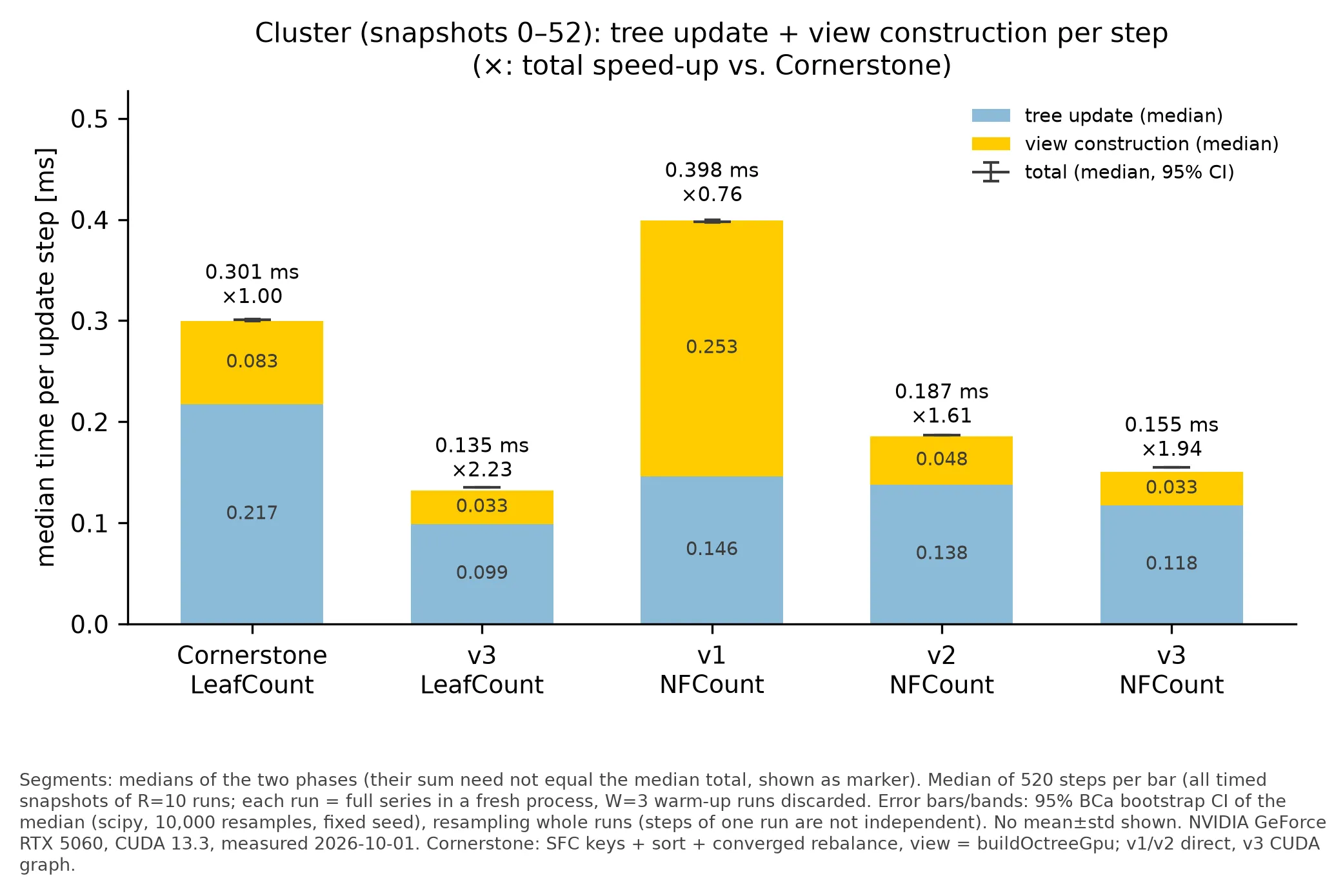
Table 3 and Figure 24 compare the final version with Cornerstone. On the small and medium time series, the LeafCount tree is built 2.0–2.4× faster while producing considerably more output. Even with NFCount, which requires 54 instead of two binary searches per fresh leaf evaluation, the construction remains 1.35–1.94× faster. On the cluster dataset, the resulting leaf arrays match Cornerstone's exactly for all 53 snapshots. The advantage shrinks for the large single-snapshot datasets. On STMV, LeafCount is still 1.16× faster, and on the 25.6-million-particle dense halo it is on par with Cornerstone, while NFCount is slower since the stencil searches dominate.

Dataset	Cornerstone	final, LeafCount	final, NFCount
Cluster simulation	0.301 ms	0.135 ms (2.23×)	0.155 ms (1.94×)
Coulomb explosion	0.405 ms	0.170 ms (2.38×)	0.221 ms (1.83×)
NaCl	0.266 ms	0.131 ms (2.04×)	0.142 ms (1.87×)
Flyby	0.978 ms	0.466 ms (2.10×)	0.725 ms (1.35×)
STMV	0.866 ms	0.745 ms (1.16×)	1.004 ms (0.86×)
Dense halo	27.87 ms	27.92 ms (1.00×)	40.67 ms (0.69×)

Table 3. Median time per step (tree update and view construction) and speedup over Cornerstone.

Note that Cornerstone converges every update completely, whereas the final version performs two passes. On the Flyby, the two trees therefore agree at only 9 of 1 201 snapshots, and the speedup compares different convergence policies.

dataset tree updateview constructionmedian total

Cornerstone

baseline · LeafCount

not measured

early September

NFCount · GPU-BFS views

not measured

mid September

NFCount · direct views, caching

not measured

final

NFCount · CUDA Graph

not measured

final

LeafCount · CUDA Graph

not measured

Medians per time step. Phase and total medians are computed separately, so the bars need not add up exactly to the tick. Speed-up relative to Cornerstone. Hover a row for details.

Median time per step for tree update (blue) and view construction (orange). Choose a dataset. The intermediate versions correspond to the repository on 3 and 10 September.

8.2 Evolution over the Project

The intermediate versions show where the speedup originates. On the cluster dataset with NFCount, the early-September version, which already produced the full FMM output on the GPU, required 0.398 ms per step (0.76× compared with Cornerstone), mostly due to the breadth-first view construction (0.253 ms). Direct reconstruction and caching reduced the total to 0.187 ms by mid September (2.1×), with the view construction alone becoming 5.3× faster. CUDA Graph execution, launch tuning and the remaining optimisations then gave another 1.2× to 0.155 ms. The Flyby follows the same pattern, from 1.93 ms over 1.14 ms to 0.72 ms. Since each version bundles several commits, the measurements do not attribute speedups to individual optimisations.

Cluster simulation: tree update and view construction per step for all implementations. · click to enlarge

8.3 Behaviour over Time

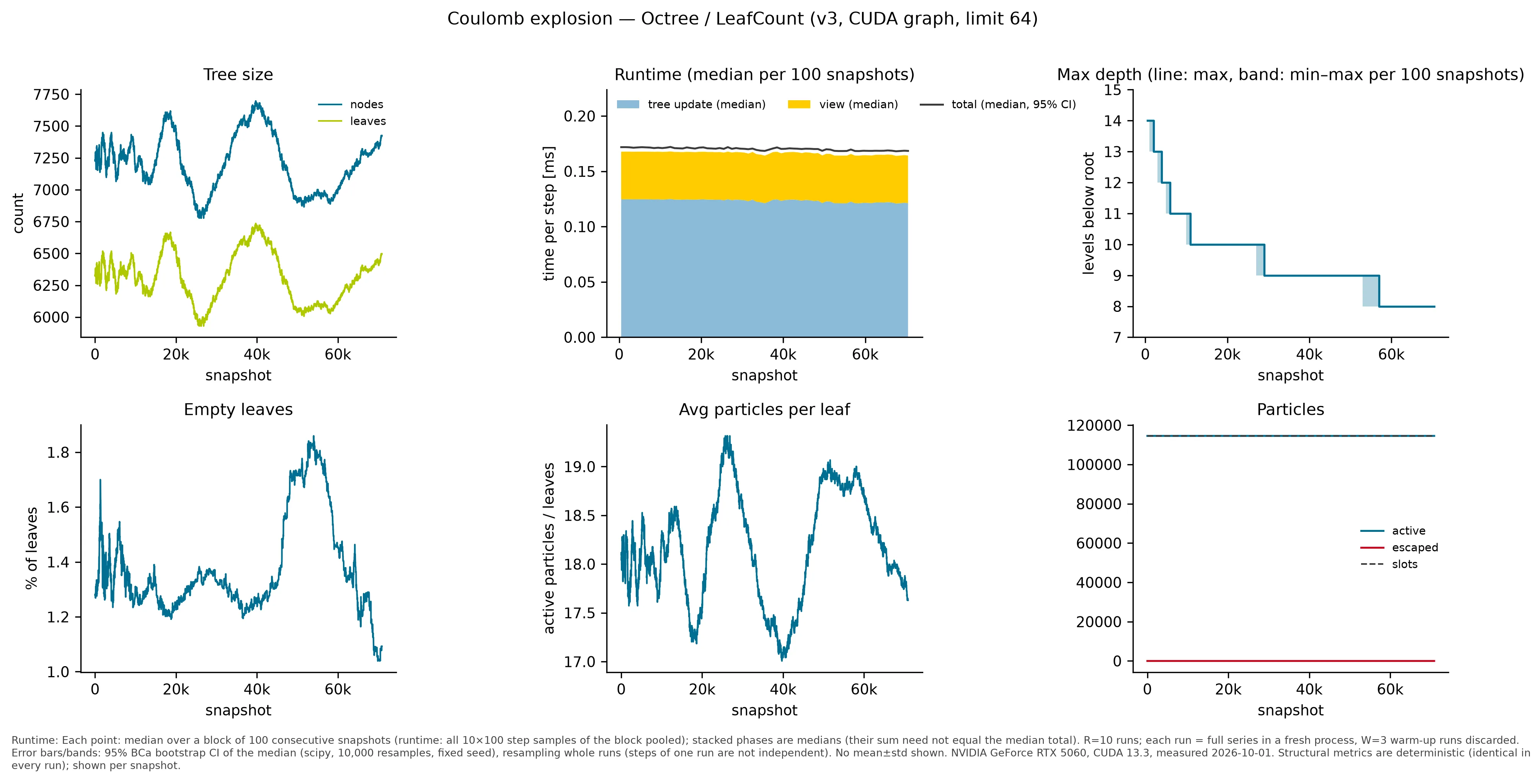
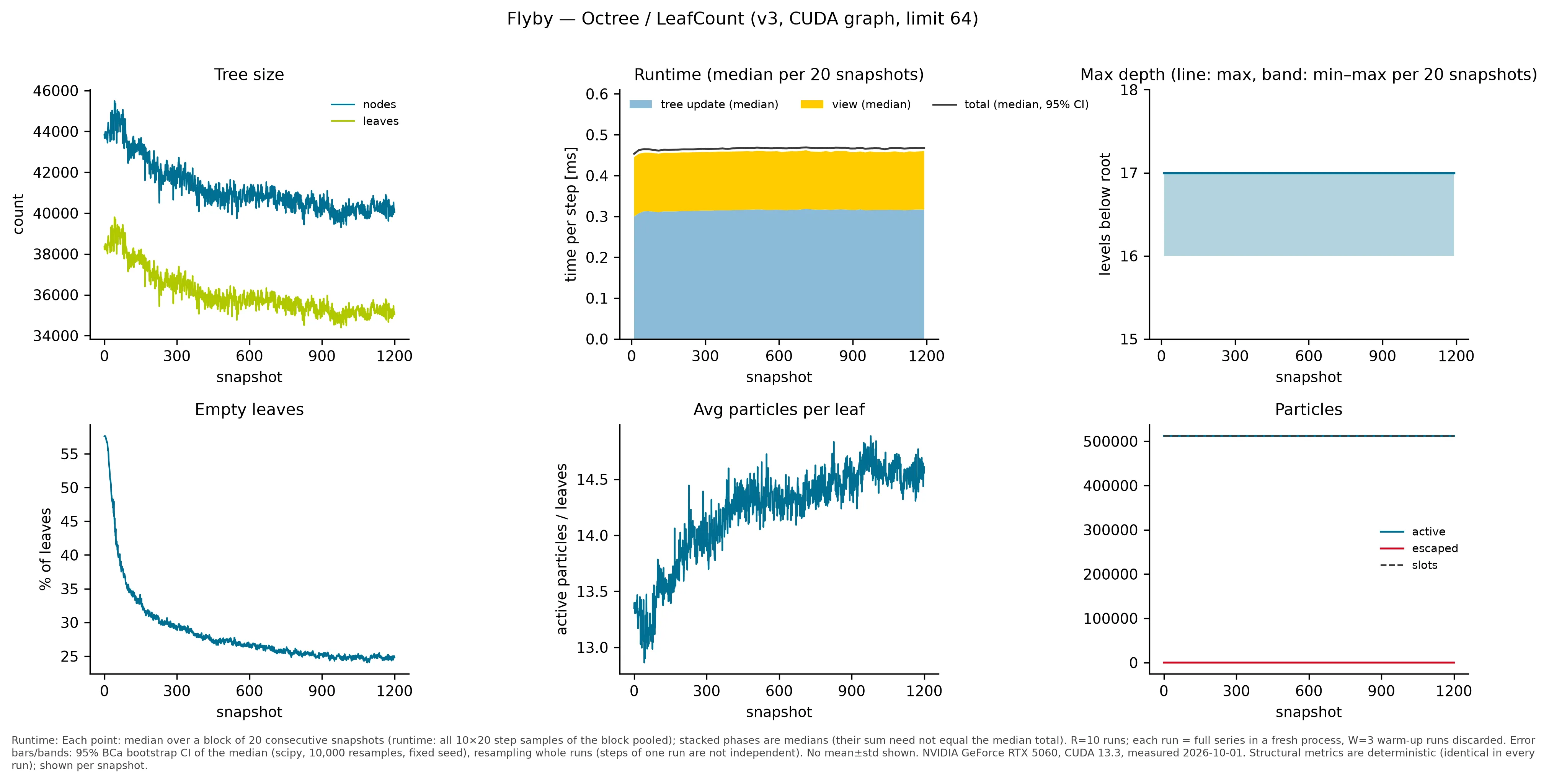
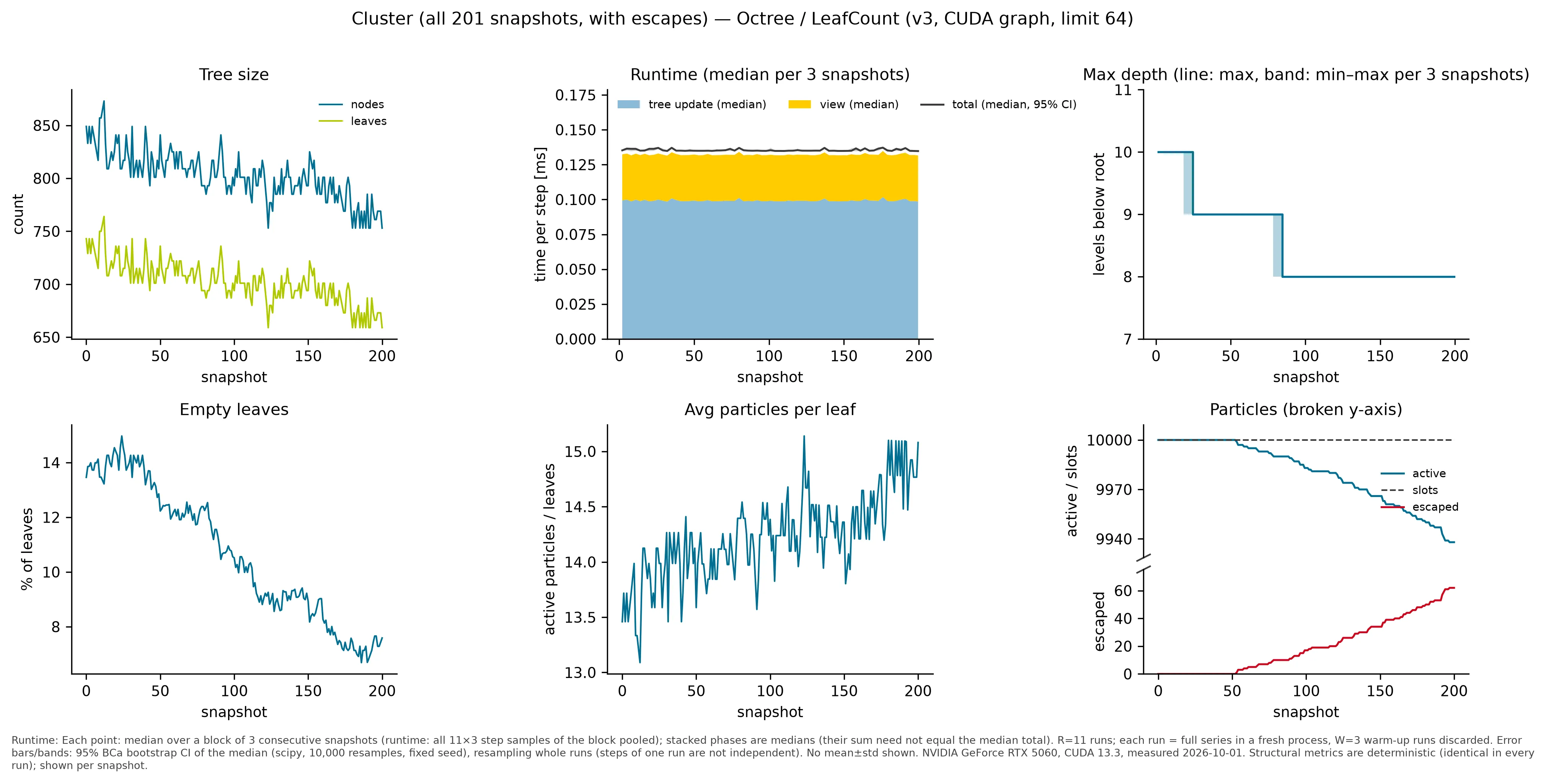
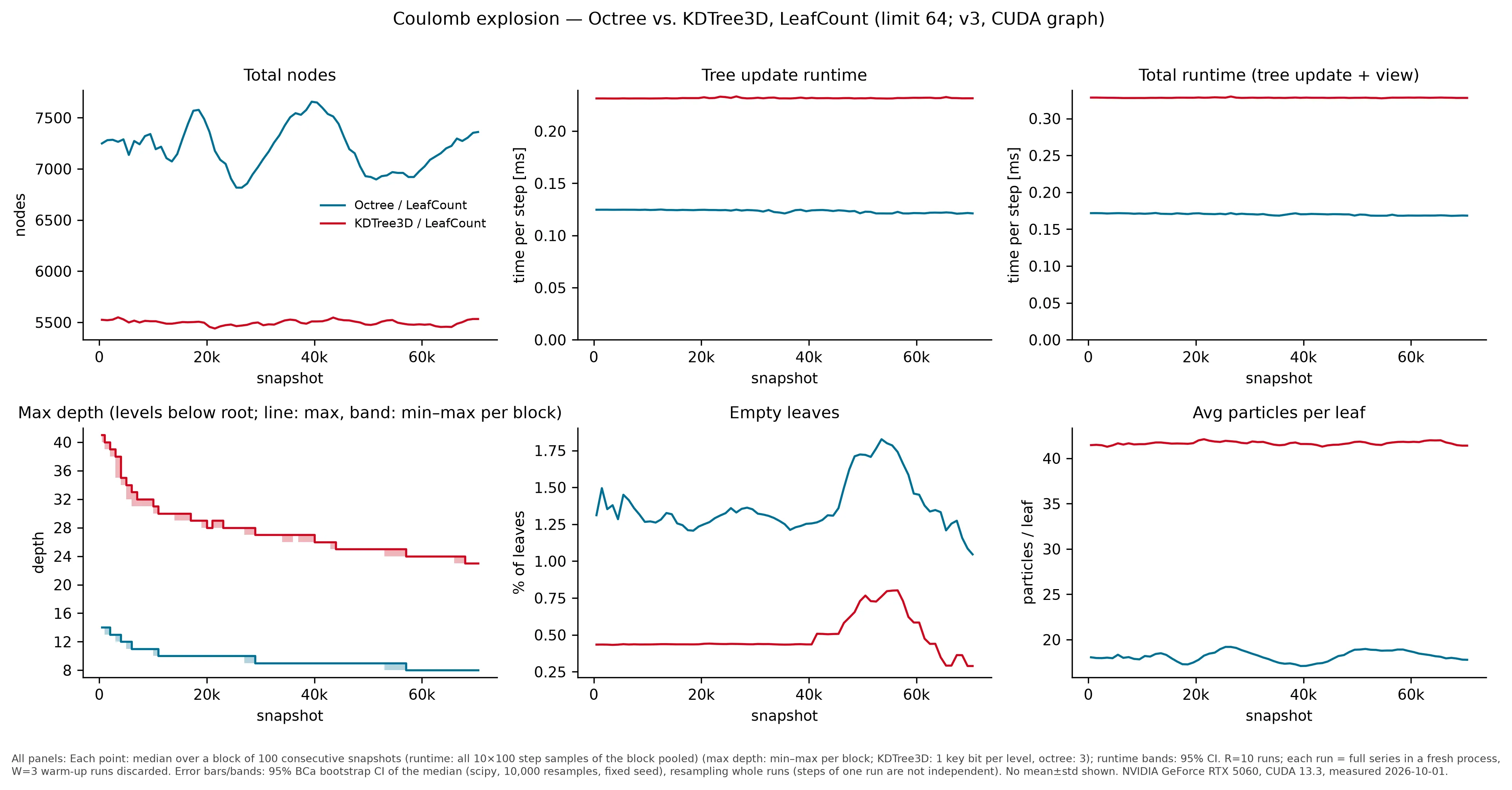
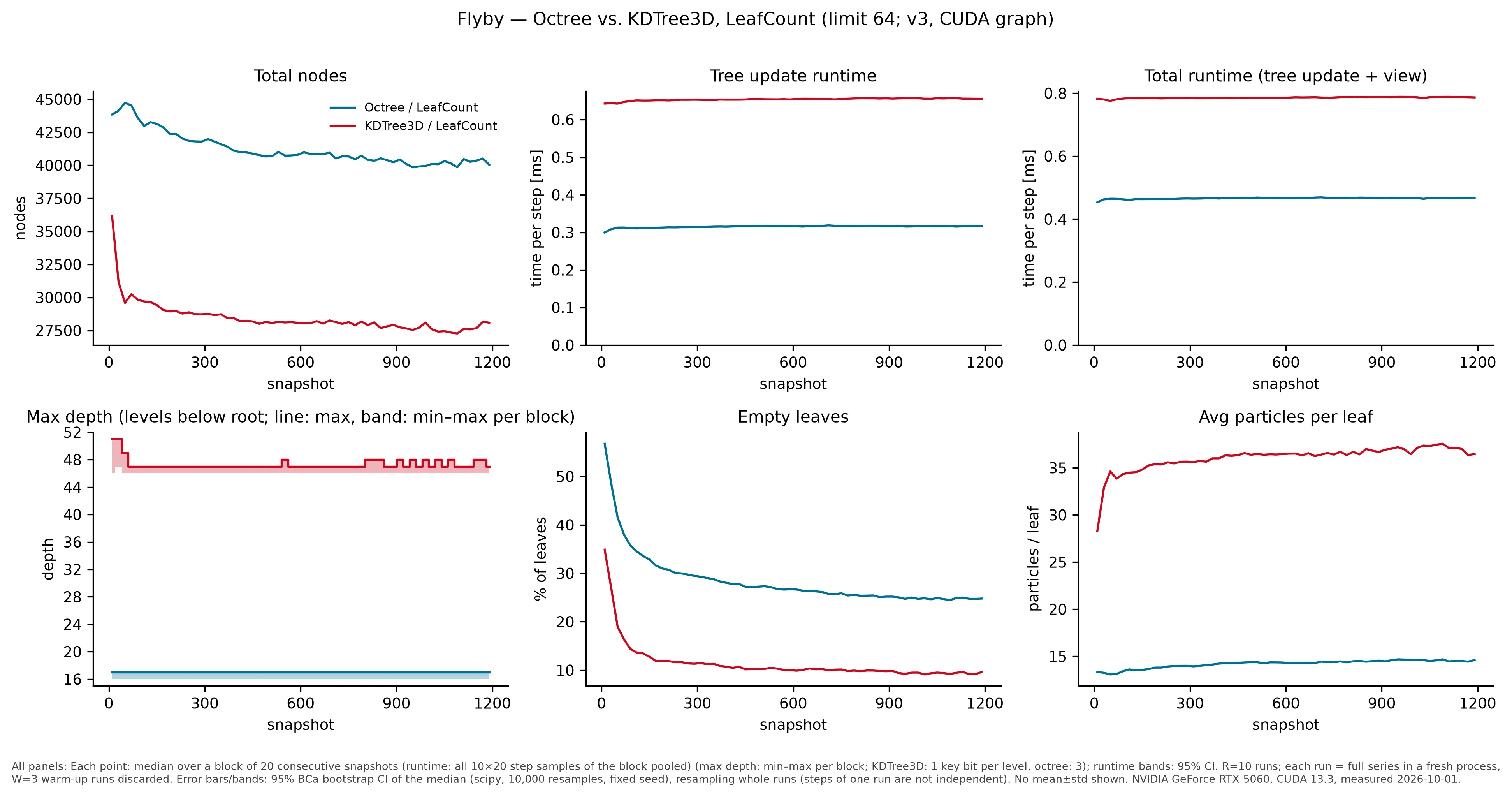
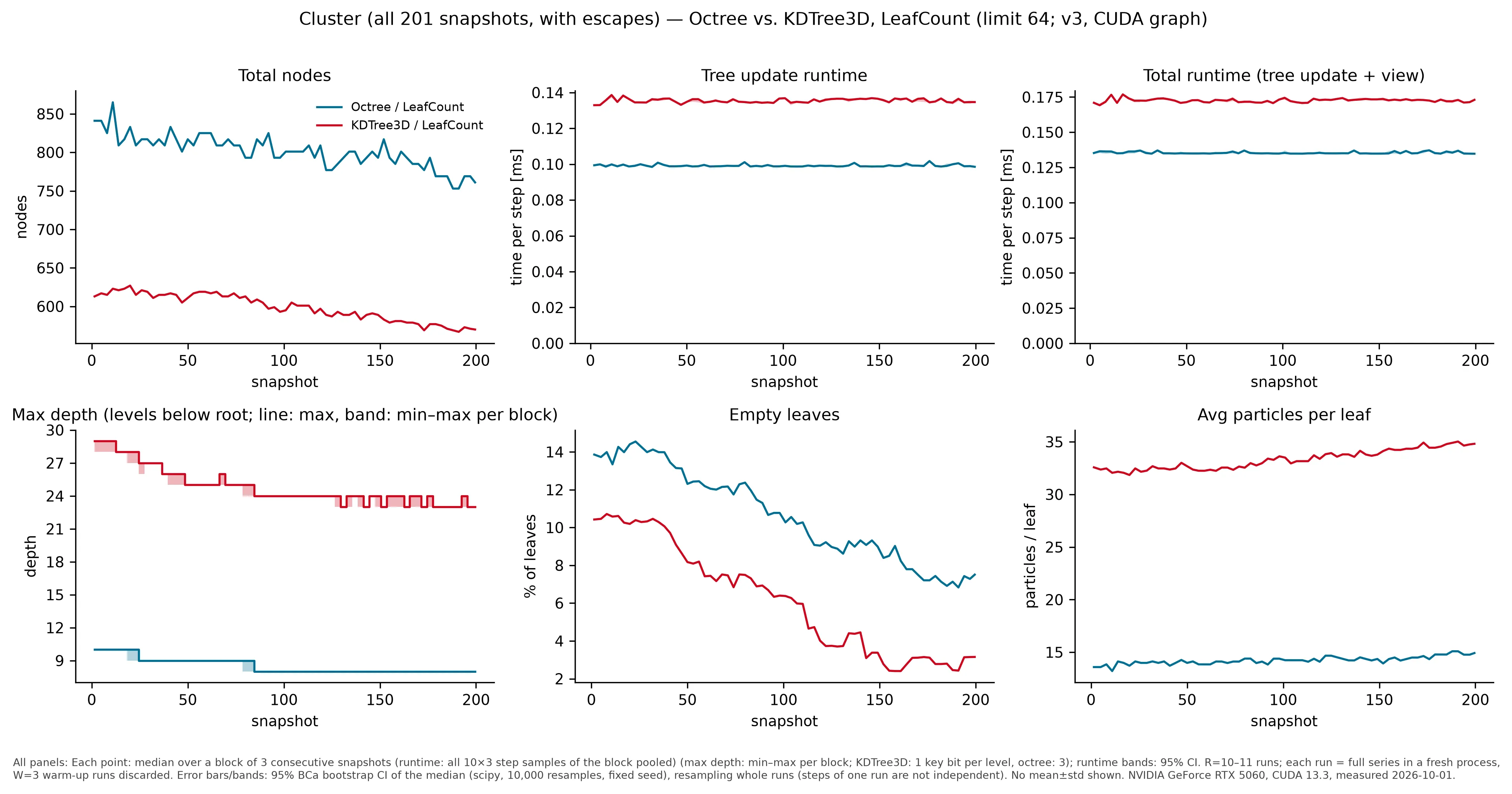
Because the update merges as well as splits, the tree size follows the particle distribution instead of only growing. In the Coulomb explosion, for instance, the maximum depth decreases as the initially dense core expands. NFCount produces more empty leaves and costs slightly more per update than LeafCount, but optimises the near-field work that the FMM performs (Figure 26). The 3D viewer in Figure 27 shows the trees themselves. In the Flyby, all particles start in a thin disk and only the centre of the domain is refined. A thousand snapshots later, the tree has followed the particles and merged cells in the centre.

figure

Coulomb explosion 114 537 particles

Coulomb explosion · Octree / LeafCount · click to enlarge

Flyby 512 002 particles

Flyby · Octree / LeafCount · click to enlarge

Cluster simulation 10 000 particles

Cluster simulation · Octree / LeafCount · click to enlarge

Top: the three time-series datasets. Bottom: per-snapshot tree statistics and runtime of the final version. Click a plot to enlarge it.

dataset

Flyby

all particles start in a thin disk, the rest of the domain stays coarse

particles

512 002

/viewer/scene-export-9.html↗

vtk.js scene · drag to rotate, scroll to zoom

Interactive 3D views of constructed trees, loaded on demand. For the dense halo, a slice through the tree shows deep levels in red and shallow levels in blue.

8.4 Full FMM Pipeline

The decisive question is whether the adaptive tree pays off inside the FMM. Table 4 and Figure 28 compare the full pipeline with a dense tree on the same inputs. For the early Coulomb explosion, the adaptive tree reduces the time per step from 11.27 ms to 2.36 ms (4.79×). The FMM phase alone drops from 11.11 ms to 1.98 ms, while tree update, view and interaction lists add only a fraction of a millisecond. The Flyby shows a similar gain (4.57×). For a small input such as NaCl, maintaining an adaptive tree costs more than it saves (0.55×), and for the halo subsample the dense tree already matches the distribution well (0.77×). Since these measurements stem from a separate harness, with means over repetitions and thresholds that changed over time, they support the overall speedup but not an attribution to individual changes.

Input	Dense tree	Adaptive tree	Speedup
Coulomb explosion, early	11.27 ms	2.36 ms	4.79×
Coulomb explosion, late	7.10 ms	2.04 ms	3.48×
Flyby	20.10 ms	4.40 ms	4.57×
NaCl	0.25 ms	0.45 ms	0.55×
Halo subsample	10.53 ms	13.60 ms	0.77×

Table 4. Full-pipeline time per step (mean over repetitions), dense versus adaptive tree.

input keys / sorttree updateviewinteraction listsFMM

dense tree

uniform depth

0.00 ms

first complete

first end-to-end version

0.00 ms

update API

tree rebuilt every step

0.00 ms

update API

incremental update

0.00 ms

newest

current version

0.00 ms

Mean time per step (separate FMM harness, RTX 5060 Ti, not re-measured with the construction benchmark protocol). Speed-up relative to the dense tree. Hover a segment.

Mean time per step of the full pipeline, split into phases. Choose an input. The intermediate rows show how the adaptive pipeline improved over the project.

8.5 Octree versus Binary Tree

Compared with the octree, the binary tree has far fewer nodes and empty leaves, more particles per leaf and a greater maximum depth (Figure 29). Its update is slightly more expensive, with 0.172 ms instead of 0.135 ms per step on the cluster dataset.

Coulomb explosion 114 537 particles

Coulomb explosion · Octree vs binary tree · click to enlarge

Flyby 512 002 particles

Flyby · Octree vs binary tree · click to enlarge

Cluster simulation 10 000 particles

Cluster simulation · Octree vs binary tree · click to enlarge

Octree (blue) versus binary tree (red), both with LeafCount, per snapshot. Click a plot to enlarge it.

9. Future Work

The main limitation concerns large dense datasets, where the 54 binary searches per leaf dominate and NFCount remains slower than Cornerstone. Reusing stencil counts between neighbouring and sibling leaves could reduce this cost considerably. A second limitation is the fixed number of passes in the graph version, which does not always reach full convergence on rapidly changing data. Adaptive pass counts and skipping capacity-sized work after convergence would address both convergence and the remaining overhead. Furthermore, $W_i$ is only a proxy for the near-field cost and ignores the far field. A calibrated cost model of the FMM operators could balance both parts more precisely. Finally, NFCount should be extended to the binary tree, and the binary tree evaluated inside the full FMM pipeline to determine when its finer granularity pays off.

10. Conclusion

This report has shown that adaptive trees can be both GPU-friendly and suited to the FMM. Storing the tree as a sorted array of space-filling-curve boundaries turns refinement into map, scan and scatter operations and makes incremental updates natural. Refining according to near-field work instead of particle density adapts the hierarchy to the work the FMM actually performs, provided that the criterion counts particles in geometric cells rather than leaves. Reading internal nodes directly off the boundary array replaces level-by-level traversal, and the reuse of work and memory together with device-owned state and CUDA Graphs reduces an update to a fraction of a millisecond. The final implementation constructs the tree up to 2.4× faster than Cornerstone and accelerates the complete FMM pipeline by up to 4.8× compared with a dense tree.

References

1. [1]H. Cheng, L. Greengard, V. Rokhlin, “A Fast Adaptive Multipole Algorithm in Three Dimensions”, Journal of Computational Physics 155(2), 468–498, 1999. doi:10.1006/jcph.1999.6355www.researchgate.net/publication/222474923_A_Fast_Adaptive_Multipole_Algorithm_in_Three_Dimensions
2. [2]S. Keller, A. Cavelan, R. Cabezón, L. Mayer, F. M. Ciorba, “Cornerstone: Octree Construction Algorithms for Scalable Particle Simulations”, PASC ’23, Article 18, 2023.arxiv.org/abs/2307.06345
3. [3]A. Lengvenis, fmsolvr-cuda (FMM code base), Forschungszentrum Jülich.code.fmsolvr.fz-juelich.de/a.lengvenis/fmsolvr-cuda
4. [4]I. Kabadshow, “The Fast Multipole Method – Alternative Gradient Algorithm and Parallelization”, Diploma thesis, TU Chemnitz; Berichte des Forschungszentrums Jülich, Jül-4215, 2006.hdl.handle.net/2128/485
5. [5]M. Dickerson, C. A. Duncan, M. T. Goodrich, “K-D Trees Are Better when Cut on the Longest Side”, ESA 2000, LNCS 1879, pp. 179–190, Springer, 2000.web.cs.ucdavis.edu/~amenta/w07/kdlongest.pdf
6. [6]L. Poirrier, “An efficient space partitioning technique based on linear kd-trees for simulation of short-range interactions in particle methods”, preprint, 2009.people.montefiore.uliege.be/poirrier/download/particle/poirrier-kdtree-pp2.pdf
7. [7]T. Hoefler, R. Belli, “Scientific Benchmarking of Parallel Computing Systems: Twelve Ways to Tell the Masses when Reporting Performance Results”, SC ’15, 2015. doi:10.1145/2807591.2807644spcl.inf.ethz.ch/Teaching/2025-dphpc/hoefler-scientific-benchmarking.pdf